April-15-2015 lab 13: Impulse - Momentum Activity

Lab 13

Purpose

Test impulse and momentum by using different experiments in elastic.

Introduction

1. Impulse

For a constant force-F, the impulse is J = F*t (average).

If F is not constant, then use the integral method to find out the J

2. Momentum

According the book, mv(final)- mv(initial).

During the collision the force is not constant. The impulse-momentum theorem states that the amount of momentum changesfor the moving cart is equal to the amount of the net impulse acting on the cart: that is J = p (change).

Experiment

This experiment is to test the idea: J = p (change) by using three different experiments.

#1: Observing Collision Forces That Change by Time.

Set up:

1. Use logPro to get the graph

2. Set up graph.

     Get the impulse acting on the cart by taking the area under force vs time graph for the collision. Measure the change in momentum of the cart by knowing its mass and measuring its speed before and after the collision using the motion detector.

3. Graph collection

     Set up all the equipment with motion detector as shown in the step 2.When everything is ready. Zero the force and begin computer graphing. Push the cart and let it collide. Repeat graphing until getting a desired graph.

4. Data analysis

 Graph result of the experiment is shown above, andit's force vs time, position vs time, and velocity vs time graphs. 

     Integral the area of force vs time, area = -0.3952N*s.

     Linear fit the velocity before the collision and velocity after. v1 = 0.3615m/s; v2 = -0.279m/s

     Calculate to test the impulse and momentum is same or not (calculation shown in the picture behind).from the picture,

In the experiment #1, the result follows the idea impluse-momentum theorem.

# 2

To test this theorem more precisely we do the same experiment as 1, but this time we increase the weight of the cart.

And then we got the graph like first one.

For this picture, we are doing the same as first.

it contains the force vs time, position vs time, and velocity vs time graphs.

After we integral the area of the force vs time, we got area = -0.6621N*s

we linear fit the velocity before the collision and velocity after. 

v1 = 0.4435m/s  v2 = -0.3622m/s

And then we do the calculation to test the impulse and momentum are same or not.

As shown in this picture, our impulse and momentum are very close to each other with errors.

Therefore, the second experiment is also follow idea impluse-momentum theorem.

# 3:

For this experiment, we give it a whole different situation than first two. When the collision, it don't go back, and it sticks on the wall.

All set up should be same as first and second, but this time we put a clay on the wall so that the cart will stop after the collision.

Using the same weight as the second experiment. m = 0.835 kg. Also, we use the same way to get our experiment done.

Give the cart a push then collect all the process. 

From this picture, the velocity will become to zero after the collision. 

it contains the force vs time, position vs time, and velocity vs time graphs.

After we integral the area of the force vs time, we got area = -0.1763N*s

we linear fit the velocity before the collision

v1 = 0.22m/s v2 = 0m/s

And then we do the calculation to test the impulse and momentum are same or not.

As shown in this picture, our impulse and momentum are very close to each other with errors.

SO we can say that for this experiment, it also follows rule.

Conclusion:

After we done three different experiments to test impulse-momentum theorem, we can say that this theorem is true for all three experiments. We can say that this theorem can be used on many those situations.

April-15-2015 Lab 12:Magnetic Potential Energy Lab

Lab 12

The purpose of this lab is to verify that conservation of energy applies to this system.

Problem: Unlike the Gravitational PE or Elastic PE, we don't have an equation for magnetic PE. So we have to find that equation.

The potential energy U is caused by an interaction force F.

So the relationship is 

So we need to find the F(r)(assume F = 0 when r approach to infinite).

Experiment 1.

To find F, we use this experiments:

We will use a glider on an aire track as our cart on a frictionless surface.

Then we raise one end of the air track the cart will end up at some equilibrium position, where the magnetic repulsion force between two magnets will equal the gravitational force component on the parallel to the track

Why we doing this experiment, because we want to find out the F magnetic. By using this experiment we can get F such that mgsin(angle) = F(magnet).

And that's how we get the F force.

And now we just need to find the angle, and the distance r from two magnets. And we assume F is some kind of power function such that F = Ar^B

We do the experiment with different angle, and get different r.

This is the data we got after trying so many different Angle, we got different r

Then we input all data into logPro. 

After we did the power fit of this line we got.

F = 0.002357 r ^ -1.349.

Experiment 2

In first one, we got F the force of magnets, now it's easy to get the potential energy

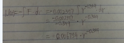
After do the change， we got U(r)

For experiment 2, we need to verify conservation energy.

We are using the set up in experiment 1, but this time we don't need to lift one side up. what we need to do it to place motion sensor on one side. And then give this cart a gentle push and record the whole time.

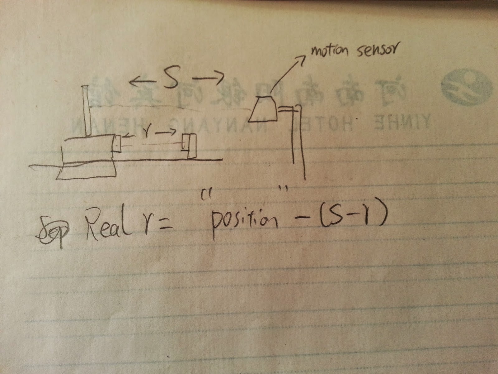
(One thing we need to care is the distance of the two magnets r, because we can see the motion sensor is not read the distance of two magnets but distance from motion sensor with board.)To find the real distance r of two magnets we difine a new column in logPro which is called real r. 

We need to do it set up the cart in somewhere, we measure the distance of two magnets r and distance of the motion sensor with the board S.

We got the real r in this experiment, and we shall use this as r.

One more thing before we start. We should set up three different column in which is PE(potential energy), KE(Kinetic energy), and total energy

PE = U（r) =0.0006754* r ^-0.3499

KE = 1/2 m * v^2 = 1/2 *0.354 * "velocity"^2

Total energy = PE + KE

Then we do the experiment, give the cart a gentle push and get the graph of PE vs time, KE vs time and Total energy vs time in one graph.

(Red one is KE, purple is PE, yellow is TE).

Uncertainty:

We can see our experiment is not perfect, because the KE should be same all the time and decrease to zero and come back with same velocity, but it's not, so the energy must change to heat, but we can assume if there is frictionless surface, you can get a perfect graph of this. 

Conclusion:

For this lab we were trying to verify the conservation of energy of two magnets. We use different experiments to get potential energy of two magnets, and use this we graph the whole thing with PE, KE, TE.Even though our experiment is not perfect, it has error or uncertainty such that the surface is not real frictionless and our measurement of U perhaps is not that close it has uncertainty on it, so those things all might affect our results.  Because of the friction, U should be started at zero but not on this experimen, and the KE should be constant and then decrease to zero and then back to same exactly position as before.

April-13-2015 Lab 11:Conservation Of Energy -- Mass-Spring System

Lab 11

Purpose: For this lab we want to show that a hanging spring with mass obey the conservation of energy.

We will be looking at the energy in a vertially-oscillating mass-spring system, where the spring has non-negligible mass.

To prove all energy is conserve, first is to find out what Potential energy and GPE of this spring.
Because the spring has mass, so function of PE and GPE will be not same like usual. Then the first part is to find out the new function

How do to find the that.
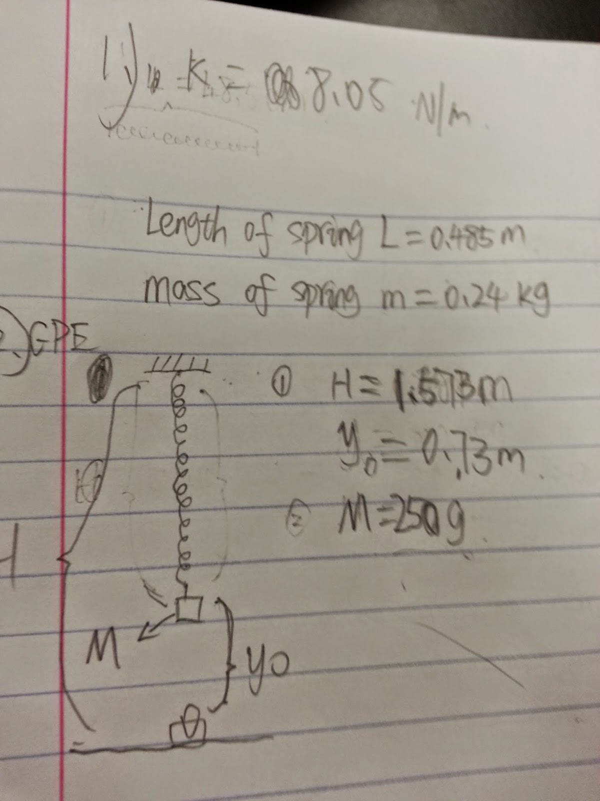
1. Choosing a representation piece dm of the pring.  dm = M/(H-y0)*dy
2. Write a expression for the GPE of that piece GPE
dm*g*y= M/(H-y0)dy*g*y.
3. Sum GPE of all of pieces of spring from y= y0 to y =H .

Then by using calculation, GPE can be written as m,spring/2* g *H + m,spring/2*g*y
Using the same method, we got KE

so that we got KE = 1/6 * m,spring * v^2

After find out the KE and GPE of this spring, then experiment can be done now.

Experiment one.

This experiment is to find out the spring constant.

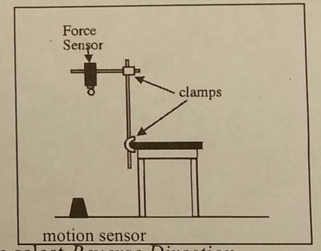
Set up all equipment like this.

Force sensor on top, motion sensor on bottom. then put a spring on the force sensor, and then zero the force sensor.

Put a 250 grams of mass on spring then start collect the data by using LogPro. 

write down the mass of the spring, length of spring when hang a mass and unstrected.



To do this experiment, push the mass on spring and then stay at some lower position. collect the whole process.

Then form the graph of force vs position. we got k = 8.05 N / m.



This is the data from first experiment.
k = 8.05N/M


H - y0 = 0.843m, This is the length when spring hang a mass M = 250 grams and unstretched.

This data will be used on next experiment.












From the first experiment, we got the constant of this spring, and unstretched length of the spring hanging a 250 grams mass, call it "stretch" = 0.843 M.

Experiment two

This experiment is the way to prove the conservation of energy.

From previous, we got KE, GPE, constant k, "stretch". One thing is missing is the elastic PE we can say it's EPE = 1/2 k* ("stretch"- "position").

Then using the same set up like before. hang a 250 grams mass on hanger, pull the spring down about 10 cm and let go. 

Then predict the graph velocity vs time, postion vs time, KE vs time, GPE vs time, EPE vs time.

and now it's time to do the real experiment. 

Open up LogPro, capture the whole process again, and get the graph of KE, GPE, and EPE vs time, postion, and velocity.

Watching from the graph, Prediction is pretty much the same as the real graph. 

Now created a new column called E(sum) = KE + GPE + EPE.

Then made a graph of E(sum) vs time.

this graph showed that Total energy is pretty much the same according to the mean and std dev of the graph. Total energy is changed very small.

Conclusion:

By using two experiment, Conservation of energy theorem is true for this experiment if there are only just KE, GPE, and EPE during the whole experiment. Of course there exists error and uncertainty such that heat or mistakes made by people, but there are still useful and truthful of this lab despite of errors and uncertainty. 

April-06-2015 Lab 10:Work-Kinetic Energy Theorem Activity

Lab 10

Purpose of this lab is to test Work-Kinetic Energy Theorem by using 3 experiments.

Experiment 1:Work Done by a Nonconstant Spring Force.

For this first experiments we want to find out the spring constant and the work done by the spring.

Set up:

(Be sure that the motion detector sees the cart over the whole distance)

Open LogPro and then display force vs position axes.

set the motion detector to "Reverse Direction", so that toward the detector is the positive direction. Then, start the cart with slowly moving towards the motion direction from the unstretched to spring is stretched about 0.2M(Depend on the spring, if it's a big spring; we can stretch it longer).

Here is the photo of the force vs position.

If we liner fit this line we got the slope of line.

For a spring we know the function f = kx, so the slope of the force vs positon is the k spring constant, so k = 1.836 N/M.

Because we know force F is change with constant. F = kx, we can calculate the work by using intergral.(We should suppose to integral from the 0 to 0.2m, so there is some loophole for this experiments, but I just want to show how to get the work.)

(This is the formula we need to calculate the work, it will start form 0 to x.)

That's also the area under the line. Therefore, we integral the line we got the Work we done by spring is 0.03243 m*N from 0.045 to 0.192M.

Experiment 2:Kinetic Energy And The Work-Kinetic Energy Principle.

For experiment 2 we want o find out the area such that we did at first one is same as the kinetic energy.

we use the same set up as experiments 1.

We get the mass of this cart is 0.573 kg.

For this experiment, we also need to use this same set up, but the different is that we need to start the cart from a stretched place and then let the cart go back the calculate the work done by the spring.

To do this experiment we need to set up a new column is that Kinetic energy which will get by 1/2 m * v^2.

We can the v by using the LogPro, and we have mass so we can get the Kinetic energy vs position graph.

Also we can get the force vs position graph either, and we can do the same experiment as 1, get the area of the graph and compare to the Kinetic energy at that point(unstretched point) to see if there are same or not.

Then we use the set up to do this experiment. 

From a stretched position and release the cart.

We choose the part where it reach to the unstretched point. rest of them just not.

So, we integral the line, we got the area is 0.07395M*N is very close to the kinetic energy 0.074 which is calculated by using 1/2 m *v^2.
uncertainty = absolute (0.074-0.07395)/0.074 *100% = 0.0675%.
so this is very close, good result.

Conclusion:

The work done by the spring is the changing kinetic energy of this spring.

Experiment 3:Work-KE Theorem.

On the above is the approximate picture of the ball.
We can calculate the work done by the ball for the whole time.

We compare our result by Work and KE, they are very close to each other but all. So the whole experiment has uncertain such that the line is not all straight ,but we ideal it, also the velocity we got is not changing of distance and time, they may have errors.

Conclusions

We have done three experiments today, First one is about the how to test the spring constant and work by a Nonconstant pull. Second one is about check the changing of kinetic energy of spring is or not the work done by the spring. Last one is about calculation.

Uncertainty of this three experiment are friction on the surface which will made the kinetic energy small.

Apr-01-2015 Lab9:Centripetal force with a motor

Lab 9

Purpose: the purpose of this lab is to find the relationship between angular speed W and the angular θ.

Apparatus:

Set up:

As show in picture, here is the equipment and set up.

To find the relationship between W and θ, we are using this equipment to set the function between them. 

Here is the force diagram and the function.

We can see the relationship between W and θ from the picture. what the lab need to do is to make sure that's true or not by experiments and then we can say that's  the relationship.

(One thing we need to know is the

 radius is not just r, it's r + R

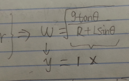
, so we got)

this function we can see as the linear

function y = kx. so the slope of this 

function should be 1 or around 1, and we can say our experiments is prove the relationship between W and θ.

Therefore, Our job is simply collect many sets of W and θ by using our equipment we just set up, then input our data into computer, linear fit the line, and see if the slope is very close to 1 or not.

How to find out the W and θ.

and W = 2PI / T

We can see H, R, and L are very easy to measure. That's the data we know.

What we need to do is to start with a slow spin at the beginning, we can measure the period by passing one specific point and get the T, then we measure the h.

By period T we can get the angular speed W, 

By knowing the h we can find the angle θ. 

Then we try with different speed, and spin the object, and then we collect the T and h.

After many tries. we got those data.

Next, we input our data in to computer, and linear fit the line.

we can see from picture, after we linear fit the data W^2 and x (which we know from above.)

We got y = 0.9827 x, so our data just prove that the relationship between W and θ is 

Uncertainty:

Of course, for every experiments we all made mistakes or errors that we cannot avoid. Our data from the experiments all have uncertainty. such that the period T

We measured or the h we got. What if our T and h are bigger, the angle will be smaller, and W will be bigger. 

Conclusion:

By trying so many times experiments, we find out the relationship between W and θ is really what we got from the function. Even though our experiments have some uncertain facts, but we can roughly say we did a very good job. For the uncertainty of this experiment, I assume that this whole experiment has no air resistance at all , and each time the small object hit on the paper, it will change the speed and direction of object. Also, the measurments I did on this experiment, such that angle, length of string or height of the paper. If I say made the whole angle I got from the experiment, W will bigger than before, or say reduce the length of string, the W will become smaller.